Square fiber using the 2D Eigen-problem solver#

[11]:

import os, sys
sys.path.insert(0,os.path.abspath('../..'))
os.path.abspath('../..')

[11]:

'/home/spopoff/dev/pyMMF'

[12]:

import matplotlib.pyplot as plt
%matplotlib inline
import numpy as np
from pyMMF.functions import colorize
import pyMMF

1. Fiber parameters#

[13]:

NA = .2
n1 = 1.45
n2 = np.sqrt(n1**2 - NA**2)
wl = 1.55 # wavelength in microns
core_size = 25 # core size in microns
areaSize = 1.5*core_size # size of the grid in microns
npoints = 2**8 # number of points in the grid

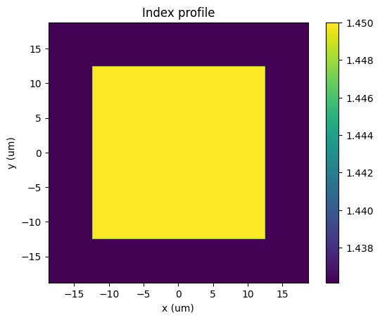
2. Create index profile#

[14]:

# Create the fiber object
profile = pyMMF.IndexProfile(npoints = npoints, areaSize = areaSize)

[15]:

index_array = n2*np.ones((npoints,npoints))
mask_core = (np.abs(profile.X) < core_size/2) & (np.abs(profile.Y) < core_size/2)
index_array[mask_core] = n1
profile.initFromArray(index_array)

[16]:

profile.plot()

3. Using the radial solver#

3.1 Estimate the number of modes#

see Comparison of round- and square-core fibers for sensing, imaging, and spectroscopy, Matthias C. Velsink, Zhouping Lyu, Pepijn W. H. Pinkse, and Lyubov V. Amitonova, Optics Express, 29, (2021)

[17]:

k0 = 2.0 * np.pi / wl
V = k0 * core_size/2 * NA
Nmodes_estim = np.ceil(V**2 / 2.0 * 4/np.pi).astype(int) //2
# note the last division by 2 is to account for we only consider one polarization
print(f"Estimated number of modes using the V number = {Nmodes_estim}")

Estimated number of modes using the V number = 33

3.2 Solve the modes with the Eigen-problem solver#

[18]:

# Instantiate the solver
solver = pyMMF.propagationModeSolver()

# Set the profile to the solver
solver.setIndexProfile(profile)

# Set the wavelength
solver.setWL(wl)

Nmodes_to_compute = Nmodes_estim+10

solver_options = {
    'boundary':'close',
    'nmodesMax':Nmodes_estim+10,
    'propag_only':True,
}

modes = solver.solve(
    solver = 'eig',
    curvature = None,
    options = solver_options
)

2024-09-10 13:11:56,225 - pyMMF.core [DEBUG  ]  Debug mode ON.
2024-09-10 13:11:56,225 - pyMMF.solv [INFO   ]  Solving the spatial eigenvalue problem for mode finding.
2024-09-10 13:11:56,226 - pyMMF.solv [INFO   ]  Use close boundary condition.
2024-09-10 13:13:04,942 - pyMMF.solv [INFO   ]  Solver found 36 modes is 68.72 seconds.
2024-09-10 13:13:04,947 - pyMMF.core [DEBUG  ]  Mode data stored in memory.

[19]:

# Be sure that we have computed enough modes
# (we discarded non-propagating modes)
assert modes.number < Nmodes_to_compute

4. Results#

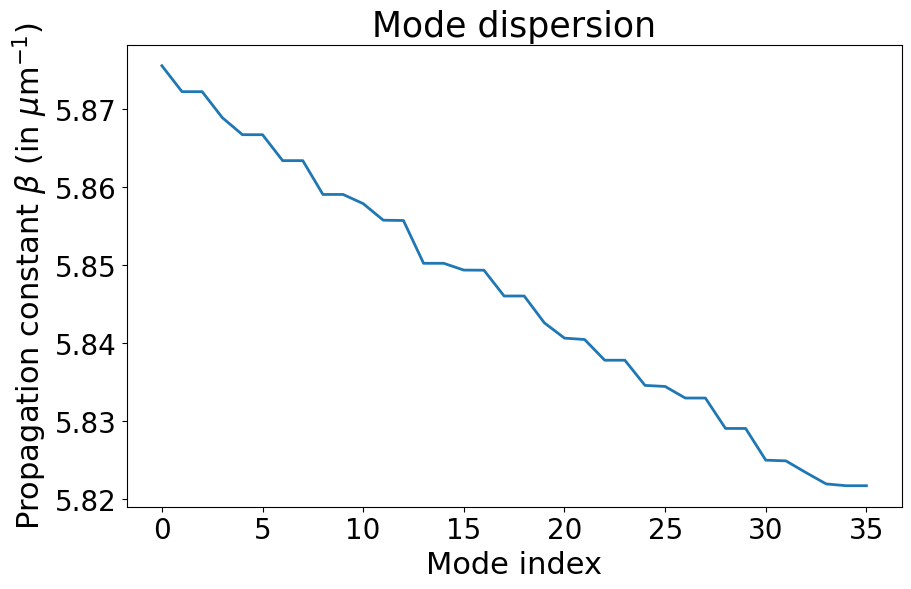
4.1 Show dispersion#

[20]:

# sort modes by decreasing propagation constant
modes.sort()

[20]:

array([ 0,  5,  2,  1,  4,  3,  8,  6, 12, 11,  7, 10,  9, 17, 15, 13, 14,
       21, 18, 16, 19, 20, 26, 25, 22, 23, 27, 24, 32, 30, 28, 29, 31, 33,
       35, 34])

[21]:

plt.figure(figsize=(10,6));
plt.plot((np.real(modes.betas)),
         linewidth=2.)

plt.xticks(fontsize = 20)
plt.yticks(fontsize = 20)
plt.title(r'Mode dispersion' ,fontsize = 25)
plt.ylabel(r'Propagation constant $\beta$ (in $\mu$m$^{-1}$)', fontsize = 22)
plt.xlabel(r'Mode index', fontsize = 22)
plt.show()

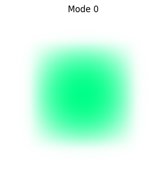
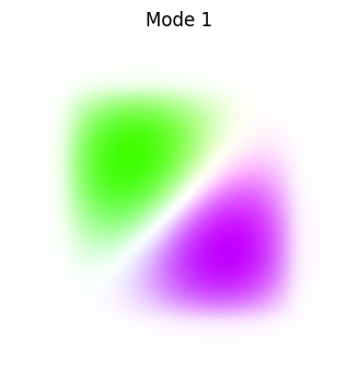
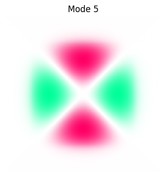
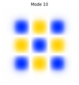
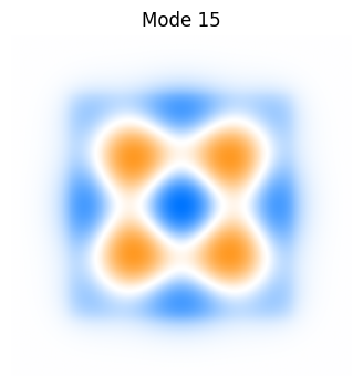
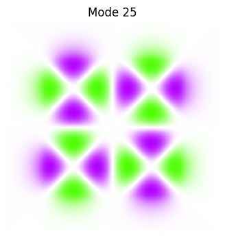
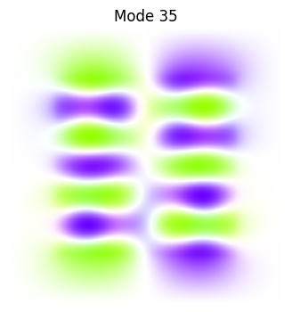
../_images/examples_Square_fiber_18_0.png

4.2 Display some modes#

[22]:

i_modes = [0,1,5,10,15,25,35]

M0 = modes.getModeMatrix()

for i in i_modes:
    Mi = M0[...,i]
    mode_profile = Mi.reshape([npoints]*2)
    plt.figure(figsize = (4,4))
    plt.imshow(colorize(mode_profile,'white'))
    plt.axis('off')
    plt.title(f'Mode {i}')